79 lines
4.0 KiB
Markdown
79 lines
4.0 KiB
Markdown
Monotonic Constraints
|
|
=====================
|
|
|
|
It is often the case ina modeling problems or project that the functional form of an acceptable model is constrained in some way. This may happen due to business considerations, or because of the type of scientific question being investigated. In some cases, where there is a very strong prior belief that the true relationship has some quality, constraints can be used to improve the predictive performance of the model.
|
|
|
|
A common type of constraint in this situation is that certain features bear a *monotonic* relationship to the predicted response:
|
|
|
|
```math
|
|
f(x_1, x_2, \ldots, x, \ldots, x_{n-1}, x_n) \leq f(x_1, x_2, \ldots, x', \ldots, x_{n-1}, x_n)
|
|
```
|
|
|
|
whenever ``$ x \leq x' $``, an *increasing constraint*; or
|
|
|
|
```math
|
|
f(x_1, x_2, \ldots, x, \ldots, x_{n-1}, x_n) \geq f(x_1, x_2, \ldots, x', \ldots, x_{n-1}, x_n)
|
|
```
|
|
|
|
whenever ``$ x \leq x' $``, a *decreasing constraint*.
|
|
|
|
XGBoost has the ability to enforce monotonicity constraints on any features used in a boosted model.
|
|
|
|
A Simple Example
|
|
----------------
|
|
|
|
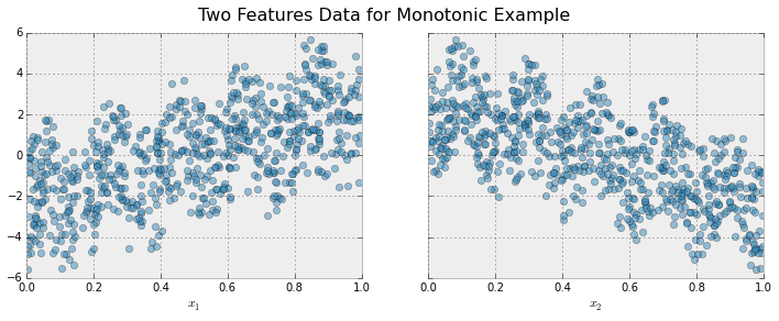
To illustrate, let's create some simulated data with two features and a response according to the following scheme
|
|
|
|
```math
|
|
y = 5 x_1 + \sin(10 \pi x_1) - 5 x_2 - \cos(10 \pi x_2) + N(0, 0.01)
|
|
|
|
x_1, x_2 \in [0, 1]
|
|
```
|
|
|
|
The response generally increases with respect to the ``$ x_1 $`` feature, but a sinusoidal variation has been superimposed, resulting in the true effect being non-monotonic. For the ``$ x_2 $`` feature the variation is decreasing with a sinusoidal variation.
|
|
|
|
|
|
|
|
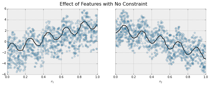
Let's fit a boosted tree model to this data without imposing any monotonic constraints
|
|
|
|
|
|
|
|
The black curve shows the trend inferred from the model for each feature. To make these plots the distinguished feature ``$x_i$`` is fed to the model over a one dimensional grid of values, while all the other features (in this case only one other feature) are set to their average values. We see that the model does a good job of capturing the general trend with the oscillatory wave superimposed.
|
|
|
|
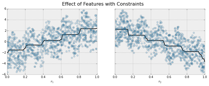
Here is the same model, but fit with monotonicity constraints
|
|
|
|
|
|
|
|
We see the effect of the constraint. For each variable the general direction of the trend is still evident, but the oscillatory behaviour no longer remains as it would violate our imposed constraints.
|
|
|
|
Enforcing Monotonic Constraints in XGBoost
|
|
------------------------------------------
|
|
|
|
It is very simple to enforce monotonicity constraints in XGBoost. Here we will give an example using Python, but the same general idea generalizes to other platforms.
|
|
|
|
Suppose the following code fits your model without monotonicity constraints
|
|
|
|
```python
|
|
model_no_constraints = xgb.train(params, dtrain,
|
|
num_boost_round = 1000, evals = evallist,
|
|
early_stopping_rounds = 10)
|
|
```
|
|
|
|
Then fitting with monotonicity constraints only requires adding a single parameter
|
|
|
|
```python
|
|
params_constrained = params.copy()
|
|
params_constrained['monotone_constraints'] = "(1,-1)"
|
|
|
|
model_with_constraints = xgb.train(params_constrained, dtrain,
|
|
num_boost_round = 1000, evals = evallist,
|
|
early_stopping_rounds = 10)
|
|
```
|
|
|
|
In this example the training data ```X``` has two columns, and by unsing the parameter value ```(1,-1)``` we are telling XGBoost to impose an increaseing constraint on the first predictor and a decreasing constraint on the second.
|
|
|
|
Some other examples:
|
|
|
|
- ```(1,0)```: An increasing constraint on the first predictor and no constraint on the second.
|
|
- ```(0,-1)```: No constraint on the first predictor and a decreasing constraint on the second.
|