7.9 KiB
Introduction to the Model of XGBoost
The Origin
XGBoost is short for "Extreme Gradient Boosting", where the term "Gradient Boosting" is proposed in the paper Greedy Function Approximation: A Gradient Boosting Machine, Friedman. Based on this original model, we incoporated several modifications to make it faster and more robust.
The General Problem
Supervised Model
XGBoost is used for supervised learning problems, where we use the training data $ x_i $ to predict a target variable $ y_i $. Our model is a mathematical structure that captures the pattern from the training data. Given the structure, we need to learn the best parameters $ \Theta $ in the model.
Loss Function
Based on different understanding or assumption of $ y_i $, we can have different problems as regression, classification, ordering, etc. To model different problems, we use a so-called loss function to describe how good is our model's performance. The function usually takes two parameters: the true value $ y_i $ and the prediction $ \hat{y}_i $. For example, we can use Rooted Mean Squared Error (RMSE)
l(y_i, \hat{y}_i) = (y_i-\hat{y}_i)^2
for a regression problem, and logistic loss function
l(y_i, \hat{y}_i) = y_i\ln (1+e^{-\hat{y}_i}) + (1-y_i)\ln (1+e^{\hat{y}_i})
for a classification problem.
Regularization
Besides we need to control the complexity of our model. A model achieving a perfect loss function score on the training dataset is overfitting it, which means it not only captures the useful pattern, but also the outliers, noise and the specific pattern in the training data. Controlling the complexity can make the model focus on more important and general pattern rather than the unnecessary details.
Optimize the Objective
Combining the loss function and the regularization, we have our objective for the supervised learning model as
Obj(\Theta) = L(\Theta) + \Omega(\Theta)
where $ L $ is the loss function, and $ \Omega $ is the regularization term. The first one is making our model being accurate, while the second one is preventing our model being overfitting. We want to have a balance between these two parts when optimizing the objective. The optimization algorithm depends on the structure of our model. The following content will introduce the details.
Boosting Trees Model
Classification and Regression Tree
The boosting trees model is a set of classification and regression trees. Here's a simple example of such a model:
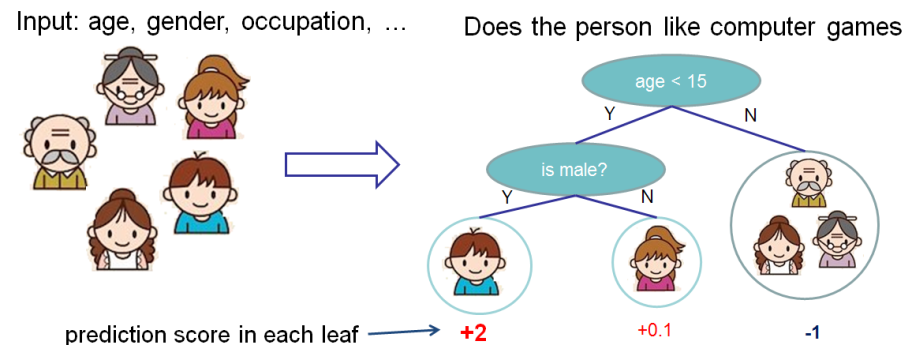
We classify the members in thie family into different leaves, and assign them the score on corresponding leaf.
Tree Ensemble
However a single CART model is not so strong in practice. How about predict with more trees?

Now we are predicting with two trees, by predict on each tree individually and then sum the scores up. Mathematically, we can write our model into the form
\hat{y}_i = \sum_{k=1}^K f_k(x_i), f_k \in F
where $ f $ is a function in the functional space $ F $, and $ F $ is the set of all possible CARTs. Therefore our objective to optimize can be written as
obj(\Theta) = \sum_i^n l(y_i, \hat{y}_i) + \sum_{k=1}^K \Omega(f_k)
Additive Training
It is not easy to train all the trees at once. Instead, we use the strategy to train them in a sequence so that everytime we train one CART and add it to the model. We note the prediction value at step t by $ \hat{y}_i^{(t)}$, so we have
\hat{y}_i^{(0)} &= 0\\
\hat{y}_i^{(1)} &= f_1(x_i) = \hat{y}_i^{(0)} + f_1(x_i)\\
\hat{y}_i^{(2)} &= f_1(x_i) + f_2(x_i)= \hat{y}_i^{(1)} + f_2(x_i)\\
\dots &\\
\hat{y}_i^{(t)} &= \sum_{k=1}^t f_k(x_i)= \hat{y}_i^{(t-1)} + f_t(x_i)
Which CART do we want at each step? Of course we want to add the one that minimize our objective.
Obj^{(t)} & = \sum_{i=1}^n l(y_i, \hat{y}_i^{(t)}) + \sum_{i=1}^t\Omega(f_i) \\
          & = \sum_{i=1}^n l(y_i, \hat{y}_i^{(t-1)} + f_t(x_i)) + \Omega(f_t) + constant
Let's consider using RMSE as our loss function
Obj^{(t)} & = \sum_{i=1}^n (y_i - (\hat{y}_i^{(t-1)} + f_t(x_i)))^2 + \sum_{i=1}^t\Omega(f_i) \\
          & = \sum_{i=1}^n [2(\hat{y}_i^{(t-1)} - y_i)f_t(x_i) + f_t(x_i)^2] + \Omega(f_t) + constant
The form of RMSE is friendly. But other loss functions could be tricky to expand. For convenience we calculate the Taylor expansion of the loss function up to the second order
Obj^{(t)} = \sum_{i=1}^n [l(y_i, \hat{y}_i^{(t-1)}) + g_i f_t(x_i) + \frac{1}{2} h_i f_t^2(x_i)] + \Omega(f_t) + constant
where
g_i &= \partial_{\hat{y}_i^{(t)}} l(y_i, \hat{y}_i^{(t-1)})\\
h_i &= \partial_{\hat{y}_i^{(t)}}^2 l(y_i, \hat{y}_i^{(t-1)})
So we can remove all the constant at the t-th step and the specific objective is
\sum_{i=1}^n [g_i f_t(x_i) + \frac{1}{2} h_i f_t^2(x_i)] + \Omega(f_t)
One of the benifit of this definition is as long as the loss function has the first and second order derivative, we can optimized every loss function within the same framework.
Model Complexity
We have introduced the details in the loss function, next we talk about the regularization term. We want to control the complexity of a tree, thus we need to define it first. We define a tree $ f(x) $ as
f_t(x) = w_{q(x)}, w\in R^T, q:R^d\rightarrow \{1,2,\cdots,T\}
where $ w $ is the vector of scores on leaves, $ q $ is a function assigning each data point to the corresponding leaf and $ T $ is the number of leaves. In XGBoost, we define the complexity as
\Omega(f) = \gamma T + \frac{1}{2}\lambda \sum_{j=1}^T w_j^2
It is possible to define other form of regularization terms, but this one works well in practice.
The best score on leaf
Now we have the objective value with the $ t $-th tree added:
Obj^{(t)} &\approx \sum_{i=1}^n [g_i w_q(x_i) + \frac{1}{2} h_i w_{q(x_i)}^2] + \gamma T + \frac{1}{2}\lambda \sum_{j=1}^T w_j^2\\
&= \sum^T_{j=1} [(\sum_{i\in I_j} g_i) w_j + \frac{1}{2} (\sum_{i\in I_j} h_i + \lambda) w_j^2 ] + \gamma T
where $ I_j = \{i|q(x_i)=j\} $ is the set of indices of data points assigned to the $ j $-th leaf. Notice that in the second line we have change the index of the summation because all the data points on the same leaf get the same score. We could further compress the expression by defining $ G_j = \sum_{i\in I_j} g_i $ and $ H_j = \sum_{i\in I_j} h_i $:
Obj^{(t)} = \sum^T_{j=1} [G_jw_j + \frac{1}{2} (H_j+\lambda) w_j^2] +\gamma T
In this equation $ w_j $ are independent to each other, the form $ G_jw_j+\frac{1}{2}(H_j+\lambda)w_j^2 $ is quadratic and the best $ w_j $ to minimize it can be solved deterministically:
w_j^\ast &= -\frac{G_j}{H_j+\lambda}\\
Obj &= -\frac{1}{2} \sum_{j=1}^T \frac{G_j^2}{H_j+\lambda} + \gamma T
Therefore, given the parameters, the gradients and the structure of the tree, we know how to set the score on each leaf.
Learning the tree structure
Our algorithm aims at optimizing the objective, so it also guides us to a good tree structure. We score the structure by $ Obj^{(t)} $ which is mentioned just above. Since we can evaluate the tree, ideally we can enumerate all possible trees and pick the best one. In practice it is impossible, so we enumerate all the trees no deeper than a certain depth greedily.
Specifically we try to split a leaf into two leaves, and the score it gains is
Gain = \frac{1}{2} [\frac{G_L^2}{H_L+\lambda}+\frac{G_R^2}{H_R+\lambda}-\frac{(G_L+G_R)^2}{H_L+H_R+\lambda}] - \gamma
This formula can be decomposited as 1) the score on the new left leaf, 2) the score on the new right leaf, 3) The score on the original leaf and 4) regularization on the additional leaf.
The regularization in the end can be seen as the minimum increment from this split. In the end, we will prune out the split with a negative gain.